
Through the Air Pays de la Loire platform, we will explore air quality to understand the complexities of the pollution problem: identifying critical areas and correlating levels with specific human activities during 2023. We will make a detailed analysis of pollutant concentration data recorded at filtered measurement stations in Loire-Atlantique. From nitrogen dioxide to PM2.5 and PM10 particles, let’s understand how these emissions affect health and the environment. Join us on this journey through revealing data that will help us better understand environmental challenges and develop solutions for a cleaner future.
Introduction
Air pollution is a major global problem. More than 6000 cities in 117 countries are monitoring air quality, but people living in them still breathe in unhealthy levels of fine particulate matter and nitrogen dioxide, with people in low- and middle-income countries suffering the highest exposures.

Pollution accelerates climate change. WHO estimates that post-pandemic air pollution is associated with more than 7 million deaths per year. Their findings highlight the importance of curbing the use of fossil fuels and taking other measures to reduce air pollution levels.
Do you know what pollutants you breathe in every day? 😷
International agencies have focused on analyzing the most common types of pollutants: concentrations of nitrogen dioxide (NO2 ), PM2.5 and PM10, and sulfur dioxide SO2.
Nitrogen dioxide (NO2 )
NO2 is a common urban pollutant and a precursor to particulate matter and ozone. It is associated with respiratory diseases, particularly asthma, leading to respiratory symptoms (such as coughing, wheezing or shortness of breath), hospital admissions and emergency room visits.
Nitrogen oxides are generated by the high temperatures of combustion processes. In places with heavy traffic, internal combustion vehicles produce about 60% of the total nitrogen oxides in the atmosphere.
The effects of these gases are obvious: reduced visibility, corrosion of materials, reduction of the growth of certain plant species, etc. In addition, they can be transformed into nitric acid which, present in the atmosphere, can give rise to acid rain in the event of precipitation.
Nitrogen oxides are largely responsible for the destruction of the ozone layer. Small amounts of these gases can destroy large amounts of ozone. This situation is aggravated by the fact that they can only be removed from the atmosphere by natural processes which are obviously much slower than the production of these gases.
Many other pollutant gases are released into the atmosphere, such as sulfur or carbon oxides, as well as other compounds and metals such as lead, cadmium, nickel, iron, mercury, chromium, copper, etc. All contribute through their negative effects on the environment.
PM2,5 and PM10
PM stands for particulate matter and the value refers to the diameter of the particles. PM2.5 is less than 2.5 microns (μm) in diameter while PM10 is less than 10 microns (μm) in diameter. Both types of particles are smaller than the width of human hair, which is typically between 17 and 180 μm in diameter.
Airborne particles, especially PM2.5 , are capable of penetrating deep into the lungs and entering the bloodstream, causing cardiovascular, cerebrovascular (stroke) and respiratory impacts. There is increasing evidence that particulate matter impacts other organs and causes other diseases as well. PM2.5 are harmful in the short term and have adverse consequences on vulnerable groups such as children and older adults. PM10, however, is more harmful with chronic and repeated exposure, especially in people with pre-existing lung disease.
Sulfur dioxide SO2
Sulfur dioxide SO2, a gas that originates mainly during the combustion of sulfur-containing fossil fuels (oil, solid fuels), carried out mainly in high-temperature industrial processes and power generation. It can cause adverse health effects such as irritation and inflammation of the respiratory system, pulmonary disorders and insufficiencies, alteration of protein metabolism, headache or anxiety, on biodiversity, soils and aquatic and forest ecosystems (can cause damage to vegetation, degradation of chlorophyll, reduction of photosynthesis and consequent loss of species) and even on buildings, through acidification processes, because once emitted, it reacts with water vapor and other elements present in the atmosphere, so that its oxidation in the air leads to the formation of sulfuric acid.
All contribute through their negative effects to the health of people and the planet itself. Therefore, all measures aimed at reducing emissions, refining, improving and optimizing internal combustion engines, or even restricting traffic in cities, are positive for our future. From the dataset obtained from the www.data.airpl.org platform, we can identify the most polluted places according to their type and the human activity that generates them.
Data source 📁
The data used on pollutant concentrations were recorded at Air Pays de la Loire measurement stations during 2023.

According to the description on the website: https://data.airpl.org/dataset/mesures, to obtain these specific data, Air Pays de la Loire implements automated particulate matter concentration measurement systems according to the NF EN 16450 standard, using two measurement methods (oscillating microbalance or beta radiation attenuation). The latter are installed in on-site measuring stations, associated with measurement data acquisition systems, which aggregate in quarterly averages. These raw data are then transmitted to the central computer server and then evaluated at different levels of aggregation (technical and environmental validations). The validated quarterly data are thus aggregated into hourly averages, which in turn are aggregated into daily, monthly or annual averages.
The information layer produced is available for use at a scale ranging from 1/250,000 to 1/10,000 and can be classified by station type:
- Traffic station: 1/10.000
- Lower station: 1/30.000 (urban) to 1/250.000 (rural)
- Industrial station: 1/100.000
Description of the fields of the data table.
- Department (/dept_name): name of the department where the measurement station is located (from IGN data).
- Municipality (/nom_com): name of the municipality where the measuring station is located (from IGN data).
- Station ( / nom_station): Name of the measurement station determined by Air Pays de la Loire.
- Pollutant (/nom_poll): name of the pollutant measured by the measurement station.
- Value (/ valeur): value of the measurement recorded for a pollutant at a given station and in a given metric.
- Unit (/unite): unit of the measured value of the pollutant.
- Indicator (/metrique): temporal aggregation level of the measured data (hour, day, month, year).
- Date / Date-time ( / date_debut): Start date of the measurement reading in local time (French metropolitan time).
- insee_com: INSEE code of the municipality where the measurement station is located (from IGN data).
- code_station: Unique code of the measuring station.
- typology(influence): Nature of the measurement station determined by its location and its influence depending on the type of pollutant it measures.
- ID_poll_ue: Identifier of the pollutant in the European reference system.
- date_fin(/date_fin) : date de fin du rapport de mesure en heure locale (heure de métropole).
- statut_valid : validité de la mesure annotée, ‘t’ si la mesure est validée, ‘f’ si la mesure est invalidée.
- X_reglementaire : coordonnée x de l’emplacement de la station de mesure à Lambert 93 (EPSG : 2154).
- Y_reglementaire : coordonnée y de l’emplacement de la station de mesure à Lambert 93 (EPSG : 2154).
Description of the method used.
According to Air Pays de la Loire, ambient air quality measurement is performed in accordance with the recommendations of the professional standards of the Central Laboratory for Air Quality Monitoring (LCSQA), in compliance with the regulatory requirements in force.
These requirements cover the entire measurement chain, both from the point of view of the criteria for establishing the measurement sites, the choice of the analysis methods implemented, the monitoring of the metrological conformity of the measurement process, the validation and aggregation of the measurement data.
Types of measuring stations
En classant la variable typologie des stations (influence), la nature de la station de mesure est déterminée par sa localisation et son influence sur le type de polluant qu’elle mesure.
Les stations de mesure sont caractérisées en fonction de leur localisation et des sources d’émission auxquelles elles sont exposées. Il existe plusieurs types de localisation (rurale, urbaine et périurbaine) et d’influence (industrielle, de fond et de trafic). Les emplacements de fond correspondent à des zones où l’exposition de la population ou de l’environnement (végétation, écosystèmes naturels) à la pollution atmosphérique est moyenne et éloignée de toute source directe d’émissions.
Methodology – Implementation of Exploratory Data Analysis (EDA)
Package installation
For the implementation of the analysis we chose Python as programming language and Google COLAB as working environment, an online tool created for the development of data science projects, integrates by default many packages widely used by data scientists.
- Matplotlib : generation of graphics from lists or tables.
- Numpy : vector manipulation software.
- Pandas : manipulation and analysis of table and time series data.
- Scipy : mathematical tools and algorithms.
- Seaborn : Statistical data visualization.
- Plotly: Online data analysis and visualization.
# Import required libraries
import matplotlib.pyplot as plt
import numpy as np
import pandas as pd
import scipy.stats
import plotly
import plotly.graph_objects as go
Importing data

Our complete data sample includes a dataset in .CSV format for each pollutant downloaded from the https://data.airpl.org/dataset/mesures platform, where it is necessary to filter the Loire-Atlantique area, each pollutant and to indicate the start and end date during 2023 with a daily periodicity.
To work with the Pandas library in our COLAB Notebook, we will import our .CSV files and convert them into a DataFrame for separate manipulation by assigning it a name (ex: so2_df), and we will also create a final dataframe (ex: df_final) that will concatenate the data of the four into one.
# We import each .CSV and convert it into dataframe with Pandas.
so2_df = pd.read_csv('so2_2023.csv', sep=';')
no2_df = pd.read_csv('no2_2023.csv', sep=';')
pm10_df = pd.read_csv('pm10_2023.csv', sep=';')
pm25_df = pd.read_csv('pm25_2023.csv', sep=';')
Data preparation
Cleaning and adapting the data for analysis is a mandatory task and may be the process where we learn the most and get the most value from the information to meet our objectives.
With the .info() command of Pandas we can obtain the number of observations, and the name, number and type of variables of each dataset.
so2_df.info()
<class 'pandas.core.frame.DataFrame'>
RangeIndex: 3648 entries, 0 to 3647
Data columns (total 18 columns):
 #   Column             Non-Null Count  Dtype
---  ------             --------------  -----
 0   nom_dept           3648 non-null   object
 1   nom_com            3648 non-null   object
 2   insee_com          3648 non-null   int64
 3   nom_station        3648 non-null   object
 4   code_station (ue)  3648 non-null   object
 5   influence          3648 non-null   object
 6   nom_poll           3648 non-null   object
 7   id_poll_ue         3648 non-null   int64
 8   valeur             3616 non-null   float64
 9   unite              3648 non-null   object
 10  metrique           3648 non-null   object
 11  date_debut         3648 non-null   object
 12  date_fin           3648 non-null   object
 13  statut_valid       3647 non-null   object
 14  x_wgs84            3648 non-null   float64
 15  y_wgs84            3648 non-null   float64
 16  x_reglementaire    3648 non-null   float64
 17  y_reglementaire    3648 non-null   float64
dtypes: float64(5), int64(2), object(11)
memory usage: 513.1+ KB
For the example of the so2_df dataset we start with 3648 observations and 18 variables available to begin our analysis. (Remember that in parallel we must do the same process for the other three datasets: no2_df, pm10_df, pm25_df, and pm25_df).
Dictionary of variables
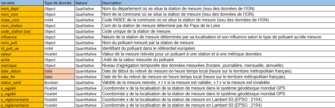
After our import, we have 18 variables of different data types. Of which 10 are qualitative and 8 are quantitative. It is important to highlight that the time variables: date_debut and date_fin are of type Object, and later we will change them to type DateTime to visualize and manipulate the data chronologically.
#Type of variable data
df_final.dtypes
output
nom_dept              object
nom_com               object
insee_com              int64
nom_station           object
code_station (ue)     object
influence             object
nom_poll              object
id_poll_ue             int64
valeur               float64
unite                 object
metrique              object
date_debut            object
date_fin              object
statut_valid          object
x_wgs84              float64
y_wgs84              float64
x_reglementaire      float64
y_reglementaire      float64
dtype: object
Preparing the data to assess its quality, we performed a check of the missing data and the proportion of null values for each variable in our set.
# What is the proportion of null values per variable in SO2 ?
(so2_df
     .isnull()
    .melt()
    .pipe(
        lambda df: (
            sns.displot(
                data=df,
                y='variable',
                hue='value',
                multiple='fill',
                aspect=2
            )
        )
    )
)
# Verification Count of null values
so2_df.isnull().sum()
nom_dept              0
nom_com               0
insee_com             0
nom_station           0
code_station (ue)     0
influence             0
nom_poll              0
id_poll_ue            0
valeur               39
unite                 0
metrique              0
date_debut            0
date_fin              0
statut_valid          1
x_wgs84               0
y_wgs84               0
x_reglementaire       0
y_reglementaire       0
dtype: int64
We can also visualize the null values inside the dataset, with this we validate that these values are not concentrated in a range of specific observations but dispersed in the dataset.
# Display null values in the whole dataset
df_final.isnull().transpose().pipe(lambda df: (sns.heatmap(data=df)))
For this example of the so2_df dataset, we have 39 observations with null values. If we analyze what information we lose by removing or imputing our missing data from each dataset, we can conclude that these null values from the four datasets do not represent a major impact on our dataset if we impute them with the mean of each variable. However, it is always important to evaluate what is the best action for these data, as they can become important outliers that change the direction of our analysis or results. I want to recommend this blogpost by Marta Castrillo that helped me a lot: How to identify and treat outliers with Python ?
📌 Note: Remember to perform the same process for the Dataset of each pollutant: so2_df, no2_df, pm10_df and pm25_df.
# We impute the variable valuer with the mean
so2_df['valeur'].fillna(so2_df['valeur'].mean(), inplace=True)
print("missing values en valeur: " +
      str(df_final['valeur'].isnull().sum()))

# We impute the variable statut_value with the mean
so2_df['statut_valid'].fillna(so2_df['statut_valid'].mean(), inplace=True)
print("missing values en statut_valid: " +
      str(df_final['statut_valid'].isnull().sum()))

Missing values en valeur: 0
Missing values en statut_valid: 0
📌 Note: If you remove null data, it is good practice to state how much data you are losing and the reason for the decision. For this case I did not remove but imputed the data, that is, I replaced it by the mean value in the variable Valuer, which is the main variable in our analysis.
Finally, we had mentioned that we should change the data type of the variables date_debut and date_fin to datetime type, for this we use Pandas again.
# Convert dates to DateTime format
so2_df['date_debut'] = pd.to_datetime(so2_df['date_debut'])
so2_df['date_fin'] = pd.to_datetime(so2_df['date_fin'])
no2_df['date_debut'] = pd.to_datetime(no2_df['date_debut'])
no2_df['date_fin'] = pd.to_datetime(no2_df['date_fin'])
pm10_df['date_debut'] = pd.to_datetime(pm10_df['date_debut'])
pm10_df['date_fin'] = pd.to_datetime(pm10_df['date_fin'])
pm25_df['date_debut'] = pd.to_datetime(pm25_df['date_debut'])
pm25_df['date_fin'] = pd.to_datetime(pm25_df['date_fin'])
It is a good practice to always check the changes, for this case we do it with .dtypes
so2_df.dtypes
nom_dept                     object
nom_com                      object
insee_com                     int64
nom_station                  object
code_station (ue)            object
influence                    object
nom_poll                     object
id_poll_ue                    int64
valeur                      float64
unite                        object
metrique                     object
date_debut           datetime64[ns]
date_fin             datetime64[ns]
statut_valid                 object
x_wgs84                     float64
y_wgs84                     float64
x_reglementaire             float64
y_reglementaire             float64
dtype: object
Before going on to perform counts and view proportions of our datasets, we are going to create or concatenate a final or general dataframe that unifies the four contaminants: df_final
# Concatenate the DataFrames into a single one per row
contaminants = [no2_df, so2_df, pm10_df, pm25_df]
df_final = pd.concat(contaminants, axis=0, ignore_index=True)
df_final.head()

# Now df_final contains the data of the 4 pollutants with the same number of columns
Descriptive statistics
Measures of central tendency and measures of general dispersion of the variable to be studied.
Of all the quantitative variables, we see that the main one to analyze is Valeur. With Numpy and the .describe method we can visualize the measures of central tendency.
# Measures of central tendency, only of numerical variables.
df_final.describe(include=[np.number])
This variable “Valeur” indicates the pollution index to be calculated as a quantitative variable.
The central variables of the df_final dataframe are defined as follows: the mean (8.485196 µg/m3) as well as the median (6.4 µg/m3).
As for the dispersion indicators, we will use the box plot to verify the level of dispersion between the mean and the median.

We note that the box plot of the variable “valeur” has its largest distribution of data between 2.2 ~ 12, presenting itself as asymmetric to the right, quite dispersed with a wide range because there are data that reach a maximum of 75.
Univariate descriptive statistics
Here we are going to extract the qualitative variables from our dataframe df_final:
# Only categorical variables
df_final.describe(include=object)
To study the qualitative variables, we will begin by visualizing the distribution by commune (commune) in Loire-Atlantique.

Thus we see that 23% of the measurements are made in the commune of Donges, then in Nantes (20%) and Saint-Nazaire (12%). If we count the observations by commune (nom_com), we can see their distribution, with Donges and Nantes as the main measurement sites. This is due to the fact that Donges is the region with the most air quality measurement stations (4 stations), followed by Nantes (3 stations), which is why it has almost twice as many observations as Saint-Nazaire in third place (2 stations).

Analyzing the Loire-Atlantique map, we can see that the Donges region has a strong industrial impact due to the presence of the Total Energies refinery, the site of a gasoline leak incident from a storage tank on December 21, 2022, which is why several monitoring and control measures were implemented on air quality in the area.

df_final.value_counts('nom_com', sort=True)
nom_com
Donges                      3646
Nantes                      3249
Saint-Nazaire               1841
Saint-Etienne-De-Montluc    1461
Montoir-De-Bretagne         1460
Frossay                     1318
Bouguenais                  1095
Rezé                         787
Paimbœuf                     365
Trignac                      365
Savenay                      364
dtype: int64
Which is the commune with the highest average concentration of pollutants?
It is important to note that when visualizing the concentration of pollutants by commune, there is no correlation between the commune with the most observations (Donges) and the commune with the highest concentration indexes, where in our case it is Rezé, followed by Nantes, which occupy the first places.
avg_concentration_by_comuna = df_final.groupby('nom_com')['valeur'].mean().sort_values(ascending=False)
plt.figure(figsize=(12, 6))
avg_concentration_by_comuna.plot(kind='bar', color='skyblue', hue='nom_com')
plt.title('Average Concentration per Commune')
plt.xlabel('Commune')
plt.ylabel('Average Concentration')
plt.show()
avg_concentration_by_comuna.head()
nom_com
Rezé                   13.108880
Nantes                 13.063650
Bouguenais             11.697341
Trignac                 8.307994
Montoir-De-Bretagne     7.894922
Name: valeur, dtype: float64
# Analysis of the concentration of pollutants by municipality in df_final
plt.figure(figsize=(15, 6))
sns.boxplot(x="nom_com", y="valeur", data=df_final)
plt.title("Concentration of pollutants by commune")
plt.xticks(rotation=45, ha="right")
plt.show()
Now it is time to analyze the distribution by “typology”: (influence), one of the most important categories of the complete data set (df_final), which allows us to establish the percentages of human activity influencing pollution in the region, according to the number of observations.

We can see that 63% of the measurements taken have an “industrial” influence. If we relate the typology with the measurement by pollutant (nom_poll) we confirm the origin of its origin.

Combining variables: bivariate descriptive statistics
The combination of variables allows us to determine whether one variable influences another.
Since the qualitative variable “valeur” is the one we want to study, we are going to perform bivariate statistics focused on this variable.

During the univariate studies, we performed a box plot on the pollutant value. It seems logical to use this plot by adding a qualitative variable to make a dispersion comparison.
We noticed that natural background and industrial stations have a similar dispersion with quantiles, medians and maxima at low levels, while specific and traffic stations have higher dispersion indicators. Again, the distribution of the stations by their influence or origin shows us that “industry” has the most observations in our data set, but it is “traffic” whose values show that it is the human activity that most affects pollution.
Therefore, we can deduce the typology that notably influences the rate of its pollutant values in each place in the region: the environments that show a high volume in “Traffic” have higher levels in pollutant values and therefore it would be advisable to avoid them to live or stay near these points.
Initiatives such as NAOAIR become important solutions to inform us in real time about the air quality, either to choose our trips or to do some sport.

For years, the European Commission has been pointing out that environmental pollution is too high and that harmful substances are shooting up above the legal limits. This EuroNews report investigates their impact in some French cities.
Most prevalent pollutants of concern:

The average concentration of pollutants shows that PM10 ☣️ is the most prevalent and therefore the most worrisome for the health of the region’s inhabitants.
Relationship between pollutant concentration and human activity by municipality:

Temporal variation of pollutant concentration per pollutant:

Calculate the measurement days and stations with the highest contamination values per pollutant:
Monitoring stations that record consistently high levels:

# Calculate the number of measurement days
num_days = df_final['date_debut'].nunique()
print(f "Number of measurement days: {num_days}")

# Identify the stations with the most pollution values.
stations_with_most_pollution = df_final.groupby('nom_station')['valeur'].mean().sort_values(ascending=False).head(5)
print("Stations with most contamination values:")
print(stations_with_most_pollution)

# Display the results
plt.figure(figsize=(12, 6))
sns.barplot(x=stations_with_most_pollution.index, y=stations_with_most_pollution.values, palette="viridis")
plt.title("Stations with Most Pollution Values")
plt.xlabel("Station Name")
plt.ylabel("Average Pollutant Concentration")
plt.xticks(rotation=45, ha="right")
plt.show()

Number of measurement days: 365
Stations with more pollution values:
nom_station
FRERES GONCOURT 17.466060
TRENTEMOULT 13.108880
LES COUETS 11.697341
CIM BOUTEILLERIE 11.027805
LA CHAUVINIERE 10.841820
Name: valeur, dtype: float64
<ipython-input-447-77ba1b50069e>:12: FutureWarning:

General trend of pollutant concentration over the last year:

# Find the most polluted day and the associated seasons
most_polluted_day = df_final.loc[df_final.groupby('date_debut')['valeur'].idxmax()]
most_polluted_day_sorted = most_polluted_day.sort_values(by='valeur', ascending=False)

Most polluted day of the year (ordered from highest to lowest value):      date_debut       nom_station  valeur
9362  2023-09-06  CIM BOUTEILLERIE    75.0
3855  2023-02-14   FRERES GONCOURT    70.0
3907  2023-02-10   FRERES GONCOURT    68.0
11651 2023-02-09        LES COUETS    66.0
1379  2023-09-08   FRERES GONCOURT    65.0
...          ...               ...     ...
11078 2023-04-02       TRENTEMOULT    11.0
9473  2023-08-27       TRENTEMOULT    10.0
1667  2023-08-15   FRERES GONCOURT     9.4
10692 2023-05-08       TRENTEMOULT     9.4
10702 2023-05-07       TRENTEMOULT     7.2

# If you also want to display the pollutant values for that day for all stations
most_polluted_day_all_stations = df_final[df_final['date_debut'] == most_polluted_day_sorted.iloc[0]['date_debut']]
most_polluted_day_all_stations_sorted = most_polluted_day_all_stations.sort_values(by='valeur', ascending=False)
Pollutant values for that day at all stations (ordered from highest to lowest value):
date_debut nom_station valeur nom_poll
9362 2023-09-06 CIM BOUTEILLERIE 75.000000 PM10
9359 2023-09-06 LA CHAUVINIERE 64.000000 PM10
9356 2023-09-06 LA MEGRETAIS 62.000000 PM10
9363 2023-09-06 TRENTEMOULT 62.000000 PM10
9358 2023-09-06 SAINT ETIENNE DE MONTLUC 61.000000 PM10
9365 2023-09-06 CAMEE 55.000000 PM10
9357 2023-09-06 FROSSAY 53.000000 PM10
9361 2023-09-06 PARSCAU DU PLESSIS 50.000000 PM10
9360 2023-09-06 LEON BLUM 48.000000 PM10
1403 2023-09-06 FRERES GONCOURT 39.000000 NO2
13408 2023-09-06 LEON BLUM 23.000000 PM2.5
13414 2023-09-06 FRERES GONCOURT 23.000000 PM2.5
13410 2023-09-06 CIM BOUTEILLERIE 22.000000 PM2.5
1401 2023-09-06 LES COUETS 22.000000 NO2
13407 2023-09-06 LA CHAUVINIERE 20.000000 PM2.5
13406 2023-09-06 SAINT ETIENNE DE MONTLUC 19.000000 PM2.5
1399 2023-09-06 PARC PAYSAGER 19.000000 NO2
13412 2023-09-06 LES COUETS 18.000000 PM2.5
13405 2023-09-06 FROSSAY 18.000000 PM2.5
13404 2023-09-06 LA MEGRETAIS 18.000000 PM2.5
1402 2023-09-06 CAMEE 18.000000 NO2
1395 2023-09-06 JULES VERNE 18.000000 NO2
1397 2023-09-06 LEON BLUM 17.000000 NO2
13413 2023-09-06 CAMEE 17.000000 PM2.5
13411 2023-09-06 TRENTEMOULT 17.000000 PM2.5
1396 2023-09-06 LA CHAUVINIERE 16.000000 NO2
13409 2023-09-06 PARSCAU DU PLESSIS 16.000000 PM2.5
1392 2023-09-06 LA MEGRETAIS 16.000000 NO2
1398 2023-09-06 PARSCAU DU PLESSIS 16.000000 NO2
1400 2023-09-06 CIM BOUTEILLERIE 14.000000 NO2
9364 2023-09-06 LES COUETS 8.448881 PM10
9366 2023-09-06 FRERES GONCOURT 8.448881 PM10
1393 2023-09-06 FROSSAY 8.300000 NO2
1394 2023-09-06 SAINT ETIENNE DE MONTLUC 7.000000 NO2
5585 2023-09-06 LA MEGRETAIS 3.500000 SO2
5592 2023-09-06 PARC PAYSAGER 1.700000 SO2
5590 2023-09-06 CUTULLIC2 1.600000 SO2
5586 2023-09-06 PASTEUR 0.650000 SO2
5584 2023-09-06 AMPERE 0.440000 SO2
5591 2023-09-06 PARSCAU DU PLESSIS 0.280000 SO2
5587 2023-09-06 FROSSAY 0.240000 SO2
5593 2023-09-06 CAMEE 0.070000 SO2
5589 2023-09-06 SAINT ETIENNE DE MONTLUC 0.000000 SO2
5588 2023-09-06 SAVENAY 0.000000 SO2The days with the highest pollution levels during 2023 were in mid-February and the first week of September, which are connected to the coldest days of winter and the week of back-to-school and back-to-vacation.
Concentration variation during different seasons of the year:

More questions 🤔
Here are some additional questions that may help us explore correlations, causality or differences that may be related to social problems linked to pollutant emissions:
- Is there a correlation between the concentration of pollutants and the rates of respiratory diseases in the population of each commune?
- Is there a relationship between industrial activity in a commune and air pollution levels in that area?
- Is there any significant difference in air quality between urban and rural areas?
- How do meteorological conditions, such as temperature and wind speed, affect the dispersion of pollutants?
- Is there evidence of socioeconomic disparities in pollutant exposure, and how does this relate to urban planning decisions?
- Does the presence of green spaces or parks in a commune correlate with lower levels of pollutants?
- Has the implementation of environmental policies or regulatory restrictions had an observable impact on the reduction of pollutant emissions?
- Can a relationship be established between urban mobility (use of public transport, electric vehicles, etc.) and air quality?
- How does public perception of air quality vary compared to objective pollution data?
- Are there differences in pollutant levels between weekdays and weekends, and how might this relate to human activity patterns?
These questions can provide a more complete understanding of the social, economic and environmental factors that contribute to problems related to pollutant emissions and air quality.
The analysis reveals critical areas of pollution in certain communes, highlighting the need for specific interventions. Correlations were identified between industrial activity, meteorological conditions and pollutant concentrations. The implementation of environmental policies and the promotion of sustainable mobility could mitigate negative impacts on air quality. In addition, socioeconomic disparity in pollutant exposure underscores the importance of addressing environmental problems from an equitable and public health-oriented perspective.
This project was undertaken with the goal of understanding the problem of environmental pollution, and putting into practice learnings in the area of data science. Needless to say, it is an exercise in personal judgment and value, and will surely be full of corrections that I hope to be able to continue to make with everyone’s feedback. 😊
Sources:
https://data.airpl.org/dataset/mesures
This EuroNews report investigates their impact in some French cities.
How to identify and treat outliers with Python ?
#qualityair #dataanalyst #LinkedInAnalysis #DataScience #EnvironmentalSustainability #pollution #climatechange #environnement #nantes #paydelaloire #loireatlantique #climat


